This is:
http://sail.zpf.fer.hr/cres/, last update 12. June 2006.
CRES
A tool for resolving of spectra of components of multiple stellar systems.
Saša Ilijić,
Dept of Applied Physics,
FER,
Univ. of Zagreb, Croatia
Contents:
Overview,
Obtaining and installing,
Example run using artificial data,
TIFR case: normalisation procedure,
Example run using real data: HD 23642,
References,
Address
For a large class of geometrically unresolved binary stars
and higher multiplicity stellar systems
one may assume that the observed spectra
are composed of time independent spectra of component stars
that add together with time dependent orbital RV-shifts,
and possibly with time dependent flux-ratii.
The observed spectra of such systems usually contain
complicated blends of spectral features of component stars
and are difficult to analyse.
The spectral separation algorithm,
introduced by [BG91] and later reformulated by [SS94], see also [H95],
takes a time series of such spectra,
together with RVs and relative flux contributions
of components in each observed spectrum,
and attempts to resolve the spectra of component stars.
The code CRES implements the spectral separation algorithm
in a very general and flexible, but computationally demanding way.
The least squares fit to the data is obtained
with the singular value decomposition technique
in the wavelength domain [SS94,I03,I04].
What makes CRES unique compared to other tools for spectral separation,
eg. [FDBinary,KOREL], is that
- each observed spectrum may cover its own spectral range,
- it may be sampled in wavelength on its own grid of points
(no regularity required),
- and each amplitude in each observed spectrum may
be weighted independently in the fit
(according to its own error-bar).
Furthermore,
- component spectra may be modeled at adjustable resolutions and
- CRES estimates errors on the amplitudes of component spectra.
Theoretically CRES can handle any amount of input data
and it can try to resolve any number of component spectra.
However, the required CPU-time is likely
to set limits to the size of the data set that can be handled.
NOTE: The so called spectral disentangling technique
goes one step further by optimising the RVs. CRES does not do that.
It is intended for critical work in spectral separation
once the RVs have been determined.
I make the code CRES available under the terms of the
GPL.
If publishing with CRES please refer to [I04]
Ilijic S, 2004,
Thoughts about disentangling in wavelength and in Fourier space,
ASP Conf Ser 318, 107-10
(preprint:
ps.gz,
pdf)
in your publication. Basically CRES consists of two files:
- cresprep.pl:
Perl script for preparing the "equations file" for CRES
- Download this file, make sure that the first line beginning with the
"#!" is the first in the file, and that the file is executable.
It is highly unlikely that Perl interpreter is not available on your machine,
but you might have to adjust its path in the "#!"-line.
- cres.c ANSI-C source file v.2.2 of June 2006
(earlier versions cres.v.2.1.c,
cres.v.2.0.c):
- To compile this source file you will have to make sure
that the GNU Scientific Library [GSL] is installed on your machine.
CRES was tested with GSL versions 1.3-1.5.
(This is the makefile
that worked fine on my i386 Linux machine,
and here is the cres executable binary file.)
Please observe comments in these two files.
In several steps I will show how to reproduce the example of
Figure 1 [PDF] in [I04].
Step 1: Prepare files with observed spectra
These are ordinary "data-files" with three numbers per line:
wavelength, amplitude and estimated error.
The files may cover a wider wavelength range
than the one that is going to be used.
The files in this example are:
c1.obs,
c2.obs,
c3.obs,
c4.obs,
c5.obs,
c6.obs,
c7.obs,
c8.obs and
c9.obs.
In this example sampling in wavelength is regular,
but note that it does not have to be that way.
Step 2: Choose spectral range and supply component RVs and LFs
The spectral range, radial velocities (RVs) and light-factors
(LFs: fractional contributions component continua
to the continuum in the composite spectrum)
must be supplied for each component and for observed spectrum.
This information is collected into one file.
In this example this cresprep.in,
see comments inside for description of the syntax.
The file cresprep.in
created in Step 2 should be processed through the
cresprep.pl script
to prepare the input file for
cres.eqs CRES.
On my computer it went like this:
   $ ./cresprep.pl < cresprep.in
   > cres.eqs
each line in the file cres.eqs,
called "equations-file",
provides all information needed to
assemble one equation of the fit.
The last line of the "equations-file"
(if created with cresprep.pl script)
specifies the total number of equations.
This is easily displayed with:
   $ tail -1 cres.eqs

   # nr of data pts (eqns) in this file: 900
Step 3: Run CRES
You may simply launch CRES and feed the input from the keyboard when asked
(your screen would look like this screen-shot),
but it is much safer and easier to prepare a simple input file
like cres.in in this example.
It is also wise to direct the screen output of CRES
into a file for later reference,
here this is cres.out.
The command line in this example is:
   $ ./cres < cres.in
   > cres.out
The calculation will, however, take some time.
Running the job in the background is recommended.
Note that cres.out is equivalent
to the screen shot shown above,
ie. it repeats all input parameters
given in cres.in.
Step 4: Examine output
The number of input files depends on the way CRES is used.
Their names are generated by appending suffices to the name of
the "equations file". In this example CRES creates the files:
- cres.out
(or the screen shot)
- The first section of this file clarifies the role
of each entry in the cres.in file.
The second section logs the calculation steps.
Here you may find an error message
if the calculation is stopped due some problem.
The third (last) section reports the results of the fit
obtained by discarding 0,1.. and so on smallest "singular values",
the last entry in cres.in
specifies how far CRES should go in discarding "singular values".
In this example discarding the smallest (first) "singular value"
lowers the chi-square relatively to the chi-square obtained
when no "singular values" are discarded.
Discarding the second one increases the chi-square again.
In a situation like this one should use the results of the fit
obtained with first "singular value" discarded.
- cres.eqs.svd
- Full sorted listing of "singular values". Ones that are
of the order of the relative machine precision should be discarded
to avoid unstable features in the fitted component spectra.
- cres.eqs.m01.s00,
cres.eqs.m02.s00,
cres.eqs.res.s00
- The model spectra for the first (suffix ".m01")
and the second (".m02") component star,
and the listing of the residuals (".res")
obtained when no "singular values" are
discarded (therefore common suffix ".s00").
In this example these files should not be used
(see discussion on "singular values" above).
- cres.eqs.m01.s01,
cres.eqs.m02.s01,
cres.eqs.res.s01
- The model spectra and the residuals corresponding to the fit
obtained with the lowest "singular value" discarded (suffix ".s01").
These should be used.
- cres.eqs.m01.s02,
cres.eqs.m02.s02,
cres.eqs.res.s02
- The model spectra and the residuals corresponding to the fit
obtained with the two lowest "singular values" discarded (suffix ".s02").
Not useful.
The format of model spectra files is:
wavelength, amplitude, estimated error.
CRES automatically distributes
the requested number of points (free parameters)
equidistantly in the logarithm of the wavelength
to cover the spectral range in which the component spectrum
can be re-constructed from the data set.
The format of the residuals file is:
obswavelength, obsamplitude, obserror,
observedminuscalcamp, hashcharacter, code.
To extract residuals corresponding to one observed spectrum,
say one with the "C3" you can use:
   $ grep C3 cres.eqs.res.s01
   > c3.res
In this example the lowest "singular value"
is of the order of the machine precision,
and is therefore considered singular,
while all other can be considered regular.
This is expected whenever the light-factors
(relative contributions of component continua to observed continuum)
of the component stars do not change with the observed spectra.
The consequence of this is that the output component spectra in
cres.eqs.m01.s01 and
cres.eqs.m02.s01
are not correctly normalised. See next section.
In time-independent flux-ratio (TIFR) case the light factors (LFs)
of the component stars do not change among the observed spectra.
The component spectra calculated by CRES are not
as such correctly normalised.
The normalisation procedure to be used with CRES,
applicable for N component spectra whose modeled
by different numbers of free parameters (wavelength points),
is coming soon.
For the special, but most useful, case of resolving two component spectra
that are modeled by the same number of free parameters (wavelength points)
the normalisation procedure [IHPF04]
formulated for the Fourier-based disentangling code [FDBinary]
can be safely used without changes.
In the paper [U04],
dealing with the distance to the Pleiades open cluster,
Munari and co-workers analysed the binary HD 23642.
They obtained five spectrograms
at Observatorie de Haute Provence, France,
with the ELODIE spectrograph in Feb. 2004.
In the Table 1 of the paper they give the component RVs they measured,
and the reduced spectrograms (deblazed flux, orders not merged)
are available at the dedicated
web page.
I use these data to provide an example of
using CRES to resolve the spectra of component stars.
Not going to undertake merging of orders,
I can separate only the central regions of individual orders.
The spectrograms are first filtered through a procedure
that removes the data points that are likely to be outliers.
Another automatical procedure
performs continuum normalisation of the spectra
in the selected spectral range.
Both procedures are very simple,
and could be significantly improved
for more critical work.
The five files
containing continuum normalised data in the
wavelength range 5160A-5180A,
extracted from the order #39 with the automatical procedures, are
Feb03_218689.obs,
Feb03_228489.obs,
Feb04_000949.obs,
Feb07_179842.obs and
Feb10_180764.obs.
The RVs corresponding to the spectra,
originating from [U04 Table 1]
are put into the cresprep.in.
Note that all light factors are set to the value 0.5,
which is in accord with the assumed TIFR [IHPF04].
CRES is run like this:
   $ ./cresprep.pl < cresprep.in
   > cres.eqs

   $ ./cres < cres.in
   > cres.out
Since we are in the TIFR case we use the output files that
correspond to the first singular value discarded.
These are the model component spectra
cres.eqs.m01.s01,
cres.eqs.m02.s01,
and the residuals
cres.eqs.res.s01.
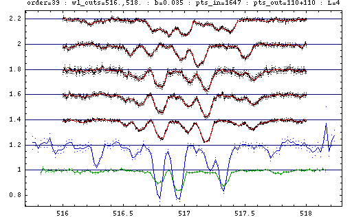
The input data are shown in black lines
with the error bars indicated by the dots one sigma above and below,
shift in the relative amplitude is applied among the spectra for clarity.
The component spectra for the brighter and the fainter component
are shown in green and blue respectively,
estimated errors shown with dots.
Component spectra are normalised using the procedure described in [IHPF04]
with the values b=0.035 for the average line-blocking in the input spectra
and L=4 for the component flux-ratio (taken from [U04 Table 2]).
The residuals of the fit are shown against the data in red colour.
This figure is available in higher resolution in PDF format:
3951605180.pdf
Procedure equivalent to the one described above was carried out
in several other spectral regions (echelle orders):
- #21 4475--4490 AA: PDF
- #33 4910--4940 AA: PDF
- #34 4945--4980 AA: PDF
- #35 4990--5023 AA: PDF
- #36 5030--5065 AA: PDF
- #37 5070--5105 AA: PDF
- #38 5120--5150 AA: PDF
- #39 5155--5195 AA: PDF
- #40 5200--5220 AA: PDF
- #61 6335--6380 AA: PDF
Please note that the results shown
are intended only for presentation of the capabilities of the code,
and are not part of other research.
| BG91 |
Bagnuolo W G, Gies D R, 1991, ApJ 376, 266
[ads] |
| SS94 |
Simon K P, Sturm E, 1994, AA 281, 286
[ads] |
| H95 |
Hadrava P, 1995, AAS 114, 393
[ads] |
| IHP01a |
Ilijic S, Hensberge H, Pavlovski K, 2001, Springer LNP 573, 269
[ads] |
| IHP01b |
Ilijic S, Hensberge H, Pavlovski K, 2001, Fizika B 10, 357
[Fizika B] |
| I03 |
Ilijic S, 2003, M.Sc. thesis
[pdf] |
| I04 |
Ilijic S, 2004, ASP Conf Ser 318, 107
[preprint:
ps.gz,
pdf]
|
| IHPF04 |
Ilijic S, Hensberge H, Pavlovski K, Freyhammer L M, 2004,
ASP Conf Ser 318, 111
[poster:
pdf,
preprint:
ps.gz,
pdf]
|
| U04 |
Munari U, Dallaporta S, Siviero A, Soubiran C, Fiorucci M, Girard P, 2004,
A&A 418L, 31
[ads, arXiv]
|
| FDBinary |
http://sail.zpf.fer.hr/fdbinary/ |
| KOREL |
http://www.asu.cas.cz/~had/korel.html |
| GSL |
http://www.gnu.org/software/gsl |
Sasa Ilijic
Department of Applied Physics,
FER, University of Zagreb,
Unska 3, HR-10000 Zagreb, CROATIA
E-mail: sasa.ilijic@fer.hr,
www:
http://sail.zpf.fer.hr/~silijic/
